Data conversion for data acquired with TS3
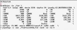
Getting the correct bruk2pipe conversion script can be tricky. The convert2pipe AU program usually doesn’t give correct results (it will interpret a 3D experiment as a 2D). It’s better to use the bruker command from a shell. Here is an example for a 3D NUS dataset that was collected with 152 hypercomplex NUS points. Type bruker in a shell:
- Set the dimension count to: 3
- Set Digital Oversampling Correction to: During Processing
- Set total/valid points in y dimension to: 4/2
- Set total/valid points in z dimension to: (eg) 152/76
- Acquisition Mode: x:DQD y:Real z:Real
- If necessary, manually enter lines to label the y dimension as Rance-Kay, and to ouput the data properly. In this case F2 was Echo-Antiecho, so we label the y dimension as Rance-Kay.
The conversion script: fid.com
Data conversion for data acquired with TS2/TS1/xwinnmr
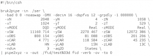
Continuing with the example from Acquiring NUS data using TopSpin 2, TopSpin 1, or xwinnmr:
An HNCACB with 64 (uniform) complex points in F1 (13C) and 55 (uniform) complex points in F2 (15N). 30% sampling gave 1058 hypercomplex NUS points in the sampling schedule. Both indirect dimensions were States-TPPI.
The conversion script can be generated either with the convert2pipe AU program or with the bruker program.
The conversion script: fid.com
Data processing
After conversion to nmrPipe format, the data processing is the same no matter which way the data was acquired.
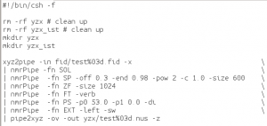
The direct dimension is processed normally in nmrPipe. The script used is ft1xyz.com:
Initially the phase values in ft1xyz.com will be 0. Run the script once, then use nmrDraw to view the first FID, which will be in the file test001.nus in the directory xyz. Each nus file has the data from one hypercomplex point. For 3D data, this will be 4 1D spectra. The first one is the one at the bottom. Phase this spectrum interactively. Then go back into the ft1xyz.com script and write in the new phase values. You can run it again to check that it’s right.
Next, run the script ft1.com. This script is almost identical to ft1xyz.com. The only difference is the way it writes out the data.
ft1.com
Now we’re ready to reconstruct the missing data. This is done with the program istHMS.
Edit the script ist.csh:
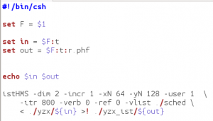
In the ist.csh script, the parameters -xN 64 and -yN 128 are the size of the two indirect dimensions after zero filling (x = F2, y = F1). These values can equal the number of (uniform) complex points in the 2 dimensions, or they can be a higher power of 2. In this case, 64 –> 128 and 55 –> 64. The only other thing you should change here is itr – the number of iterations that the istHMS program does. It will be faster with fewer iterations, but the quality of the reconstruction may degrade. 400 iterations is usually enough.
This script starts the istHMS program. It uses the sched file, which is the schedule of NUS points that your experiment ran. Unfortunately, the 2 columns of the sched file are often in the wrong order. All of our 3D NUS experiments are done with aqseq 321. So F2 is the “first” indirect dimension, and F1 is the “second” indirect dimension. Therefore, the correct order of the columns in the sched file is:
F2 F1
In other words, the column on the left should be the vplist (the F2 NUS points), and the column on the right should be the vclist (the F1 NUS points). If they’re in the wrong order, you must swap the columns. You can delete (or rename) the file sched. The files vclist and vplist are in your data directory. There is a script called sched_combine_vp_vc.py that will make a new sched file with the vc/vp lists in the proper order.
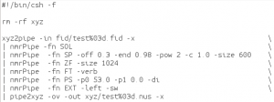
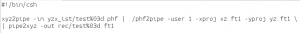
The run the script run.local, which starts the script ist.csh and istHMS:
![]()
This does the recontruction and writes the files test*.nus into the directory yzx (* = 001, 002, etc)
Now run the script phf2pipe.com. This reorders the data into planes (back into the format that nmrPipe expects).
phf2pipe.com
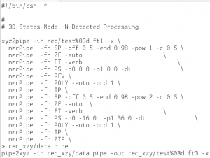
Now that the reconstruction is done, the 2 indirect dimensions can be processed normally by nmrPipe:
An example processing script for F1 and F2: ft23_xyz.com
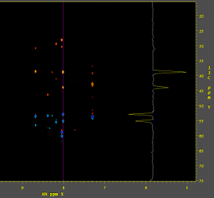
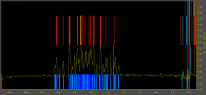
You can view the data in nmrDraw:
Processing scripts
You can get processing scripts from the Wagner lab website. There are also example processing scripts and executables in the directory /home/peterson/NMR/NUS/Processing_Scripts:
fid.com (there are different versions of fid.com for different types of experiments)
ft1xyz.com
ft1.com
run.local
parallel
sched_combine_vp_vc.py
ist.csh
istHMS
phf2pipe.com
phf2pipe
ft23_xzy.com
Remember that you may have to modify some of these – especially the nmrPipe conversion and processing scripts.