SMILE: Sparse Multidimensional Iterative Lineshape-Enhanced reconstruction of NUS data
SMILE is a new (2017) NUS processing algorithm published by Jinfa Ying, Frank Delaglio, Dennis Torchia, and Ad Bax.
Ying, J., Delaglio, F., Torchia, D.A., and Bax, A. J. Biomol. NMR 68(2): 101-118 (2017)
It is provided as a plug-in to nmrPipe. It must be installed along with nmrPipe, and requires a version of nmrPipe posted October 14th 2016, or later. More information can be found here.
Data Conversion
*Note: All data processing instructions that follow assume familiarity with nmrPipe processing.
The data conversion is best done using the bruker program that is supplied with nmrPipe. The only thing that’s necessary for the bruker program to recognize your dataset as an NUS dataset is that a file called nuslist exists in the data directory. If you’ve acquired the data using TS2, just rename the file sched to nuslist.
Here are three examples of data conversion:
Example 1: 2D HSQC acquired using TS3 50% sparcity
Starting in your data directory, type:
>bruker -nus -nouseMask
This will bring up the usual GUI, with NUS features added:
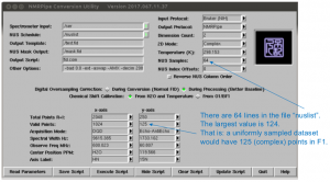
All the important information, including all the NUS information, will be read in automatically when you click “Read Parameters”. You’ll probably have to adjust the usual things like “Center Position”.
This will generate a script (fid.com) which does the data conversion:
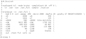
Example 2: SMILE used as an alternative to linear prediction to extend a constant time
SMILE can also be used to predict data points at the end of uniformly sampled data. For example, to extend a constant time. It works much better than linear prediction, and it’s very easy to implement. The conversion is done exactly as the conversion of any normal (ie, not NUS) dataset:
>bruker
This will bring up the GUI, but without the added NUS stuff. It will generated the usual fid.com script:
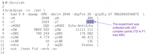
Example 3: 3D HBHAcoNH acquired using TS2 25% sparcity
Rename the sched file to nuslist and start the bruker GUI:
>mv sched nuslist
>bruker -nus -nouseMask
As before, click “Read Parameters” in the GUI, and adjust things like the “Center Position”. It will generate a conversion script (fid.com) appropriate for a 3D dataset acquired using NUS:
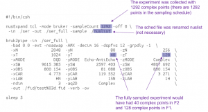
Run the conversion script:
>./fid.com
Data Processing
One very nice feature of the new bruker conversion is that it sorts and expands the NUS data into a larger matrix (the size that the uniformly sampled dataset would have been), and places zeros into the not-sampled points:
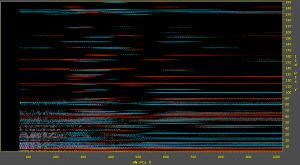
Sorted and expanded data from 50% sparse HSQC
The data can then be processed normally (with no reconstruction). This is exactly like processing any normal (not NUS) data using nmrPipe.
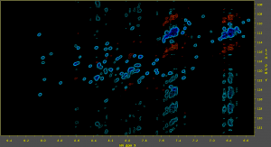
50% sparse NUS HSQC, processed with no reconstruction
The spectrum processed this way has many artifacts, but the peaks are clearly visible. The correct phase values can be found this way. This is important because the correct phase values must be known for the reconstruction to work properly.
Reconstruction is done in nmrPipe using the new function SMILE. This is illustrated using the same three examples as above:
Example 1: 2D HSQC acquired using TS3 50% sparcity
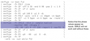
The direct dimension is processed first, then a transpose is done to place the indirect dimension first. Then the SMILE reconstruction is done on the indirect dimension, then the indirect dimension is processed. Notice that the phase values for the indirect dimension also appear in the SMILE reconstruction.
*One non-standard thing in this script is that the value of the parameter xT is 250. This parameter controls by how much the original data is extended. The default value is 0. If “-xT 0” is set, then the data in the reconstructed dimension will be extended by 50% (the default). In this case, there were 125 complex points collected (but 50% sparse, of course), so it would have been extended to 187 or 188 points. I wanted more resolution, so I set “-xT 250” to force it to extend out to 250 complex points. That is – in addition to filling in the missing points in the the first 125, it also uses SMILE to fill in (or predict) 125 additional points.
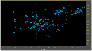
Reconstructed HSQC acquired with 50% sparcity
Example 2: SMILE used as an alternative to linear prediction to extend a constant time
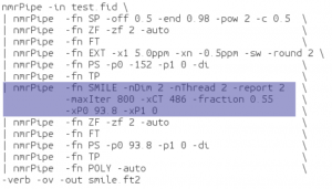
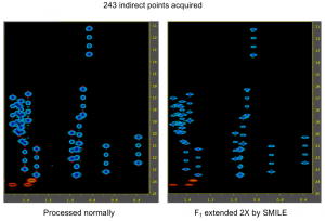
In this case, the spectrum was uniformly sampled, so there is no nuslist. However the SMILE function used with the parameter xCT set to 486, tells it to use SMILE to extend the original 243 complex points out to 486 complex points. Again, the indirect dimension phases must be set during the reconstruction as well as during the final processing.
Example 3: 3D HBHAcoNH acquired using TS2 25% sparcity
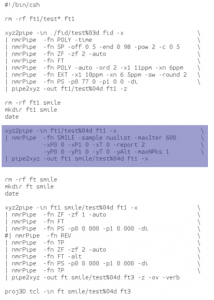
As with 2D data, with 3D data the direct dimension is processed first. The data is then reordered so that XYZ becomes YZX. Or the original Y and Z dimensions (the 1st and 2nd indirect dimensions in nmrPipe-speak) are moved into the X and Y positions. Then the SMILE reconstruction is done, then the two indirect dimensions are processed. For a 3D dataset, there are “x” and “y” phases, as well as xT and yT parameters. Here, “x” refers to the first indirect dimension and “y” refers to the 2nd indirect dimension. The phase corrections should exactly match the two sets of phase corrections for the two indirect dimensions that appear below the SMILE reconstruction in the script (here they’re all zero). “-xT 0” and “-yT 0” tell it to use the default 50% extension in both indirect dimensions.
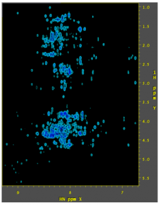
F1-F3 projection from reconstructed HBHAcoNH spectrum